Helpful Tools in Data Manipulation
 Basic Tools
- Freezing Panes
How to Freeze Rows or Columns in Excel?
Step 1. Select the row below the row or rows that you want to keep visible. If you prefer to freeze columns, you must select the cell to the right of the column that you want to freeze. Step 2. Go to the View tab. Step 3. Select the Freeze Pane dropdown and choose “Freeze Panes.” You can use this video as your guide in freezing your row or column: https://www.youtube.com/watch?v=ki9bY4oLVMc Sorting Data Sorting your data helps you to reorganize your spreadsheet quickly. For instance, you can sort your list of products by its suppliers. You can also sort it numerically, alphabetically, and in many other ways. Before sorting the data, you must first decide if you want to sort the entire spreadsheet or just a particular column. Sort sheet Sort sheet allows you to organize all of your data based on one column. Related information across each row is remained after the sortation. It is the best one for you if you want to arrange your data alphabetically or alphanumerically. Sort range Sort range is ideal for a sheet with several tables. It sorts the data in a variety of cells without affecting the other content on the worksheet.Are there any Expert Techniques to Manipulate Data in Excel and Increase Efficiency?
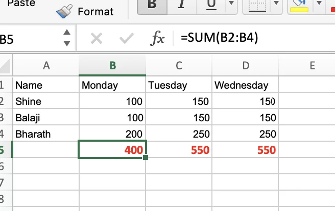
Using efficient typing techniques in handling data with Excel can greatly enhance productivity. Operations like swift copying and pasting are made easy through keyboard shortcuts such as Ctrl+C and Ctrl+V. Effective data management can be attained by using formulas and functions like VLOOKUP and SUM. Skillfully applying sorting and filtering options allows for prompt organization and analysis of data. Grasping these sophisticated tactics allows users to maximize their efficiency in Excel to its full potential.
Can Excel Techniques be Applied to Create CSS Graphs and Charts?
Yes, Excel techniques can indeed be applied to create CSS graphs and charts. By using CSS and HTML, you can apply styling and formatting to the graphs and charts created in Excel, making them visually appealing and interactive. With the help of css graphs and charts tutorials, you can learn how to incorporate CSS techniques into your Excel graphs and charts, enhancing their overall design and functionality.
How to sort a sheet?
Step 1. Select the cell in the column that you want to sort. Step 2. Click the data table, choose the Sort 7 Filter group, and do the following: To sort in ascending order, click the A-Z button To sort in descending order, click the Z-A button in descending order. You must not forget to check if all data is sorted as text. If you want to sort a column that contains numbers, you can format them either number or text. You can choose your sorting option in the Format Cells dialog, click the Category dropdown and select your preferred sorting option. You can use this video as your guide in sorting your data:Function Tools
Here are some of the essential functions or formulas in manipulating data.IF Statements
If statements are useful for several situations. It can save your time and output a text if a particular data is valid or false. For instance, you can write the function =IF(A1>A2, “EXCELLENT”, “FAIL”), where A1>A2 is the case, “EXCELLENT” is the output if true and “FAIL” is the output if false.SUMIF, COUNTIF, AVERAGEIF
All of these functions or formulas are structured like =FUNCTION(range, criteria, function range). So in SUM, you can put =SUM(A1:A10, “EXCELLENT”, B1:B10). This function will automatically add the values of B1 to B10 if the total sum of A1 to A10 has an output of “EXCELLENT”. You may be starting to think that these functions can make your complex spreadsheets easier.MAX and MIN
These functions may be simple, but they are sure to help a lot when you have a massive amount of data. For example, you can put =MAX(A1:A10)if you want to get the maximum numerical value in those rows while you can use MIN to find the minimum.AND
AND is one of the widely-used logical functions in Excel. It automatically checks if certain things are true or false. For instance, =AND(A1=”EXCELLENT”, B3>10) would output true if A1 is “EXCELLENT” and the value of B3 is greater than 10. You can add more value by simply adding another comma per value. Other Excel functions that you must know:| FUNCTION | USE |
| =Average(A1:A10) | Calculates the average of a set of data |
| =Count(A1:A10) | Counts the number of cells in a range that contain numbers |
| =CountA(A1:A10) | Counts the number of cells in a range that are not empty |
| =Large(A1:A10,n) | Returns the nth largest value in a data set |
| =Product(A1:A10) | Multiplies a range of data |
Auto Filter
AutoFilter is one of the effective ways to find your data faster. Excel has several filter options that you can use to subset the information on your spreadsheet The categories are:| CATEGORY | USE |
| Simple Numeric Conditions (Equals, Does Not Equal, Greater Than, etc.). | If you select one of these options, Excel will open up a dialog box in which you can specify up to two simple numeric conditions. |
| Top 10… | Display rows containing the top N values. |
| Above Average | Display numeric values that are above the average value. |
| Below Average | Display numeric values that are below the average value. |
| Custom Filter… | This opens up the same dialog box as you get when selecting the individual Numeric Conditions (Equals, Does Not Equal, etc.), to allow you to specify up to two numeric conditions. |
Can I Use Excel to Create Interactive Infographics?
Yes, you can use Excel to create beautiful interactive infographics technology trends. By using features like data visualization, charts, and interactive elements, Excel can be a powerful tool for creating engaging infographics that showcase the latest technology trends in an interactive and visually appealing way.
How to apply the AutoFilter?
Step 1. First, click the range of cells that you want to filter. Step 2. Click the Data tab and select the Filter option The dropdown menu will be visible on each of your header cells. It can be used to display specific rows for a particular category.VLOOKUP Function
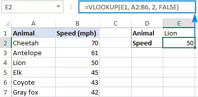
You can you VLOOKUP to search and retrieve data from a particular column in the table. It supports exact, approximate, and even wildcards. The letter “V” stands for “vertical”. It helps you to search through your data while basing on your unique identifier. Here is an example of the VLOOKUP function: What are the things to remember in using VLOOKUP?
- The VLOOKUP function can only search in the leftmost column of a table and returns a value from a column to the right. This function cannot look at its left. If you need to look for values from the left, you can use the INDEX MATCH combination since it does not care about lookup positions and return columns.
- The VLOOKUP function is case-insensitive. Therefore, both lowercase and uppercase characters are treated equally. If you want to distinguish data with case sensitivity, you can you the VLOOKUP case sensitive formulas.
- Remember the importance of TRUE and FALSE in the last parameter. You must use FALSE if you are looking for the exact match while TRUE for the approximate match.

